More on Gaussian Processes
This part of the course continues the discussion on Gaussian Process (GP) surrogate models from Part 3 and provides an introduction to the theory of Gaussian processes. This theory forms the foundation of GP regression and GP surrogate models.
Gaussian Processes
GP surrogate models are based on regression, or fitting, of data to Gaussian processes. A Gaussian process is an infinite collection of random variables, any finite number of which have a joint Gaussian distribution. In practice, we will only ever work with finite collections of random variables. Consider a series of  random variables with Gaussian, or normal distribution. We can view these variables collectively as a vector of random values:
  . Such a vector can be visualized as a discrete function with linear segments drawn between each point. Each visualization below shows five samples for vectors of length
  and
and  , respectively, with each variable in the vector having standard Gaussian, or normal, distribution of mean
  and variance
  (standard deviation
  ). If these variables
  are all independent, or uncorrelated, then there is no structure to the vector, and we get a "white noise vector". Each y-value (circle) in these graphs corresponds to the value of one of the random variables plotted versus the index
  . Each time we generate, or draw, a random sample vector, we get a new "function".

Five random vectors of length 10 with uncorrelated Gaussian random variables viewed as functions of the vector index.

Five random vectors of length 100 with uncorrelated Gaussian random variables viewed as functions of the vector index.
If we now introduce correlations between the different variables in the vector, we get something that is more useful as a function to use for regression purposes. The visualizations below show five samples for two vectors of length and , respectively, with so-called squared exponential correlation and zero mean value. This is the type of function that is used as a basis for GP regression. As we increase the length (or density) of the vector, we see more of the correlation structure.

Five random vectors of length 10 with Gaussian random variables correlated with a squared exponential covariance.

Five random vectors of length 100 with Gaussian random variables correlated with a squared exponential covariance.
One of the main ideas behind using Gaussian processes for regression is that we can roughly speaking think of a function as a long vector. Instead of using a discrete set of indices , we can use a continuum of indices and we can let this continuous index be time  , the spatial coordinate
  , or some other variable, such as temperature, stress, or voltage. The theory requires us to think of a Gaussian process as a vector of infinite length, however, in practice we only look at vectors or finite length. In this way, we get functions
  with a certain covariance function
  , also called covariance kernel, that takes as input any pair of real values. For example, in the function plots above the following squared exponential covariance function was used:

where  is the signal variance, which determines the vertical scale, or amplitude, of the functions, and
  is the correlation length, which determines the horizontal scale of the functions; how quickly the functions are allowed to vary. The signal variance and correlation length are commonly referred to as hyperparameters since they control the overall behavior of the surrogate model.
A probabilistic way of understanding the correlation length, , is that it that determines how quickly the correlation between neighboring points decays. In a random vector, that we view as a kind of discretized function, we typically want neighboring variables and  to have a stronger correlation than, say, the first and last variables
  and
and  in the vector. This behavior is controlled by the covariance function which determines how much neighboring points are "co-varying". Similarly, in the continuum case, points that are close together should have a stronger correlation in order to produce interesting functions that can be used to fit physical data. We measure the distance between points as:

and we can see that the squared exponential covariance function can alternatively be written in terms of  as:
as:

A covariance function that only depends on the relative distance between points is called a stationary covariance function. Otherwise it is called a nonstationary covariance function.
Note that when  , that is, when we measure the correlation of a point with itself, the value of the covariance function equals the signal variance and corresponds to the strongest level of covariance. For large values of , the exponential function is close to zero, indicating a very low level of covariance for points that are far apart. Also, note that if we let the correlation length approach zero, we recover a white noise process with no correlation (the covariance function becomes a Dirac delta generalized function).
Visualizing Gaussian Process and Gaussian Multivariate Distributions
Consider one function for the case of a vector of length 100. The proper mathematical language to describe such a function is that it is a random sample drawn, or realized, from a Gaussian process with zero mean value and squared exponential covariance function.

One random vector of length 100 with Gaussian random variables correlated with a squared exponential covariance.
For practical purposes, here we look at only 100 of these dimensions, which corresponds to the 100 random values in the vector that we plot as a function. In other words, one way of visualizing a randomly drawn point from this infinite dimensional probability distribution is to view it as a continuous (technically almost) function. A Gaussian process is an infinite dimensional generalization of a multivariate Gaussian distribution function. A function that is randomly drawn from its distribution is equivalent to a random point sampled from this infinite dimensional distribution.
It is difficult to directly visualize a multivariate Gaussian distribution function in 100 variables. To build intuition, we can instead visualize a joint distribution in the much simpler case of two variables with points drawn at random from such a distribution. Let's say that we have a joint Gaussian distribution for two variables  , with zero mean vector and unit variance. This joint distribution function can be visualized using color, as shown below.

A bivariate joint Gaussian distribution function.
If we now draw random sample points following this joint distribution, we get a scatter plot that resembles the corresponding distribution function plot with a higher density of points where the probability distribution function values are higher:

A set of 10,000 randomly sampled points from the bivariate Gaussian distribution.

The same set of 10,000 points colored uniformly.
As above, we can visualize points sampled from this distribution as vectors, or functions. These samples correspond to discrete functions with values at only two points, corresponding to the two random variables (or x and y coordinates of the points in the figures above). The figure below shows five sample vectors.

In general, a function that is randomly drawn from a Gaussian process corresponds to one sample point but drawn from a high-dimensional distribution.
Gaussian Process Regression
Let's now consider the continuous case. The following visualization shows five sample functions drawn from a Gaussian process with a squared exponential covariance function and zero mean, defined over the interval [0,1], sampled at evenly distributed points:

Five functions drawn as realizations (or samples) from a Gaussian process with a squared exponential covariance function and zero mean.
These sample functions are allowed to vary within the boundaries of what the given mean value and covariance function admits. The probability distribution, defined by the mean value and covariance function, of these functions is referred to as the prior distribution in GP regression.
Let's say that behind the scenes we have an unknown function that we will approximate using GP regression, based on very little information in terms of very few measurements. We will successively reveal more and more information in forms of data points  , called training points, to the regression process. To begin, let's say we know just one value of the unknown function, for example,
  . Knowing one value allows us to change the background GP probability distribution into a constrained version of the original distribution, called a conditional probability distribution. This new process is more constrained compared to the original Gaussian process, which is free to vary wildly. This conditioning of the probability distribution essentially corresponds to removing one of the dimensions from a multidimensional normal distribution. In a real simulation case, such a training point would come from the output of some quantity of interest of a finite element simulation (or other numerical simulation). The following visualization shows five functions drawn from this conditional Gaussian process using approximately 200 test points. A test point is simply a point that is not in the known, or seen, dataset. In other words, a test point is where we try to predict the value of the unknown function.

Five functions drawn as realizations (or samples) from a Gaussian process with a squared exponential covariance function and zero mean.
As can be seen from the plot, knowing the value at just a single data point still allows the sample functions to vary widely, except near its known value, making it difficult to make good predictions without additional data.
We can repeat this process. Assume now that we know the value at two training points, as shown in the figure below:

Five functions drawn as realizations (or samples) from a Gaussian process with a squared exponential covariance function and zero mean, conditioned on the value at two points.
Repeating again, now for six training points, the drawn GP functions appear as follows:

Five functions drawn as realizations (or samples) from a Gaussian process with a squared exponential covariance function and zero mean, conditioned on the value at six points.
We can see from these plots that the GP functions show less variation where we have more information, i.e., where we have more known data. This phenomenon can be used to determine the uncertainty of the fit. Where there is more variation in the sample functions, there is more uncertainty. We can also understand that one of the assumptions behind the uncertainty estimate when using GP regression is that the unknown variations are Gaussian (normally distributed), but with certain covariance properties. This assumption is reasonable for a wide variety of practical cases.
Next, for each x-coordinate, we can take the mean value of a large number of realizations, or samples, of the Gaussian process, and in that way get a prediction, together with uncertainty, of the unknown function. This mean value function is what constitutes a GP surrogate model. The figure below shows the mean value of the corresponding conditional Gaussian process; the original Gaussian process conditioned on the values at the training points:

The mean value function of the Gaussian process based on knowledge of six data points.
We can see that the unknown function appears to be a sine function. Indeed, the presumed unknown function is  . In the next section, we will study how well the original function is approximated by the GP regression.
Gaussian Process Mean and Variance
In a practical GP regression implementation, such as the one in COMSOL®, the mean value function is derived analytically from the covariance function and the training data, as outlined in the course part More on Gaussian Process Surrogate Models. There is no need to generate a large number of Gaussian process sample functions. The mean value function is a result from the regression process and corresponds to a conditional Gaussian process mean analogous to a conditional multivariate distribution mean. For GP regression, although we may assume a prior distribution with constant mean, the output posterior distribution typically has a nonzero and spatially varying mean. In the discrete case, we can view the mean function as a long vector:  , or as a mean function
  .
.
Similar to the mean function, the uncertainty is analytically represented in terms of variance,  , when considering a single point. When considering multiple points, the uncertainty corresponds to a covariance . The analytical expressions for the GP mean and variance correspond to the conditional mean and covariance of the multivariate Gaussian distribution formed by the training and test points. Specifically, this refers to the distribution of the test points (the points we aim to predict) conditioned on the location and values of the training points (the points we know).
For a derivation of the conditional mean and covariance, see C.K. Williams and C.E. Rasmussen, "Gaussian processes for machine learning", MIT Press, Cambridge, MA, vol. 2, no. 3, p. 4, 2006. This derived distribution is known as the posterior distribution. Note that the term "GP prediction" is sometimes used interchangeably with "mean function." The ability to view the regression process as a conditional distribution of a Gaussian process allows for a well-defined uncertainty to be associated with the function fit. This level of uncertainty definition is not as easily achieved with other methods, such as radial basis function (RBF) fitting, discussed in our resource detailing More on Gaussian Process Surrogate Models.
Although the background Gaussian process corresponds to an infinite dimensional Gaussian distribution, since we are always interested in the value at a finite number of test points and training points, in practice, we only ever need to handle a finite dimensional distribution. Furthermore, due to the fact that the background process is infinite dimensional, GP models are sometimes referred to as nonparametric models. However, in this context, nonparametric rather means that the model has an infinite number of parameters.
The visualization below shows the variance estimate around the mean function of the example above, expressed as one standard deviation, colored in grey.

The variance around a GP regression mean function, expressed as one standard deviation.
To appreciate the power of a nonparametric model, compare it with fitting data to a piecewise polynomial. In the case of a piecewise polynomial model, you need to decide a priori on the number of intervals and the polynomial degree. If the model is not sufficiently accurate, you need to increase the number of intervals and/or the polynomial degree manually. In contrast, with a nonparametric GP model, the complexity of the model automatically adapts as you add more training data. This allows the GP model to capture more complex patterns without the need for explicit adjustments to the surrogate model structure.
Visualizing a Conditional Distribution
To further build some intuition behind GP regression, let's consider its interpretation as a conditional probability distribution. Slicing a joint Gaussian distribution function along one of the coordinate axes gives a conditional distribution. The conditional distribution function is also a Gaussian distribution function (bell curve) and represents the probability density function for one variable given a certain value of the other. For example, given  we get the following one-variable distribution function when conditioning a two-variable distribution:
 A square that displays a rainbow color distribution in a slanted-like radial direction, going from dark red near the center to dark blue at the edges, with a red line that slices through the square.
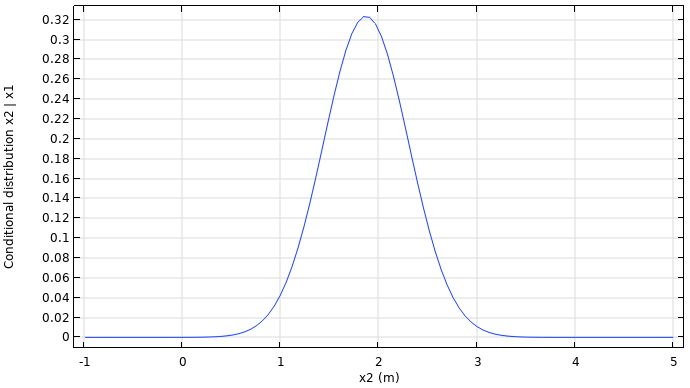 A graph consisting of a blue line that displays a parabolic curve pointing downwards that gradually flattens out with x2 on the x-axis and the conditional distribution on the y-axis.
Slicing the bivariate normal distribution along an axis gives a conditional distribution function for one of the variables.
This is analogous to GP regression since the process of constraining the Gaussian process using six points, as shown in the earlier example, corresponds to conditioning the Gaussian process distribution function for six variables. However, this 6-dimensional cut takes place in a higher dimensional space. Note also that although the sample functions may all have a zero, or constant, mean vector, the conditional distribution will typically have a spatially varying mean vector, or, rather mean function. In the example above, the fitted mean function (or we can see it as a long mean vector) is certainly nonzero and is indeed spatially varying.
Submit feedback about this page or contact support here.