Learning Center

Choosing the Space Dimension and Physics Interfaces

---

The most important decision in defining a magnetohydrodynamics (MHD) model in the COMSOL Multiphysics^® software is choosing the space dimension to work in and which of the electromagnetic physics interfaces to use in the model. This is because identifying a combination that minimizes the number of degrees of freedom that have to be solved for in the model can significantly decrease the amount of computer memory and time required to solve the model.

Identifying which space dimension and physics interfaces are required can be done by examining the symmetries of the system, the expected direction of the induced current in the fluid, and the sources of the electromagnetic fields.

Choosing the Space Dimension

Three space dimensions are available for MHD modeling in COMSOL Multiphysics^®: a full 3D formulation, a 2D cross-section formulation, and a 2D axisymmetric formulation. For each problem it is necessary to identify which of these formulations is most suitable. The 2D models are preferable when possible because they involve significantly fewer degrees of freedom due to the smaller geometry and fewer mesh elements, although 3D modeling is the general approach. However, strict restrictions on geometry and physics must be met in order to use a 2D formulation.

Using a 2D Axisymmetric Formulation

The 2D axisymmetric formulation is designed for the case where both the geometry and physics are rotationally symmetric around a central axis. In this case, cylindrical coordinates are used and the and components of the field are solved for. The model is solved for on a cross section taken through the r-z plane. The 2D solution can be revolved to form the full 3D solution.

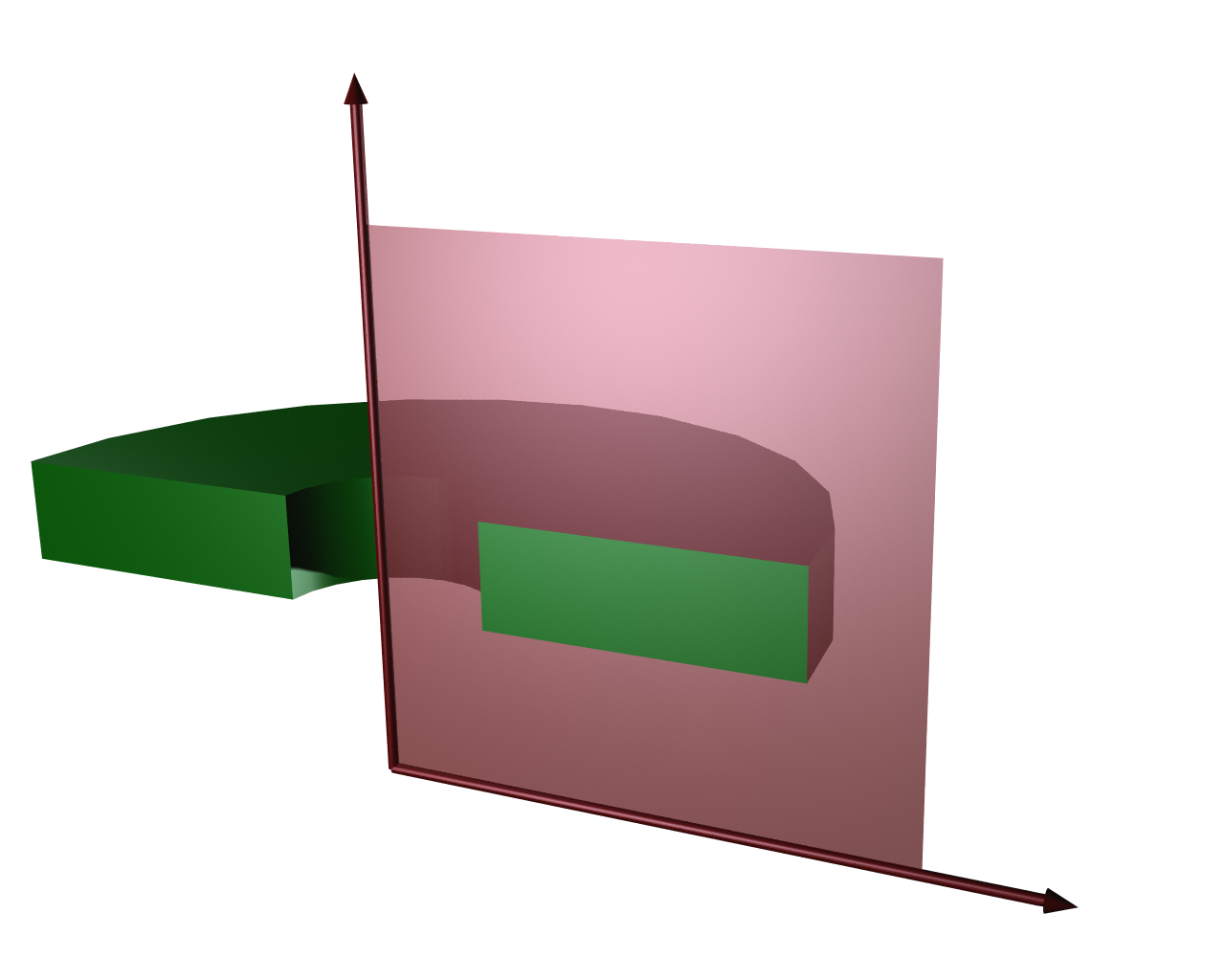
The modeling plane used in the 2D axisymmetric formulation (red) and its relationship to the full 3D geometry (green).

In COMSOL^®, certain physics interfaces, including the fluid flow interfaces, have stricter requirements for using them for axisymmetric modeling than the standard requirement that the physics is rotationally invariant. The requirements to use a 2D axisymmetric model for MHD modeling are:

• The geometry has to be rotationally symmetric.
• The fluid flow has to be rotationally invariant, and either the flow has to be entirely in-plane, or any out-of-plane flow has to be handled under swirl flow. This allows for out-of-plane flow, which is:
  • Driven by a force or wall motion
  • Applied with a boundary inlet that includes an in-plane flow component
• The magnetic and electric fields and the current have to be rotationally invariant. There is no restriction on their in-plane and out-of-plane components.

The 2D axisymmetric formulation is useful for modeling the flow or pumping of conductive liquids through cylindrical pipes, rotational velocity monitors, and other similar systems.

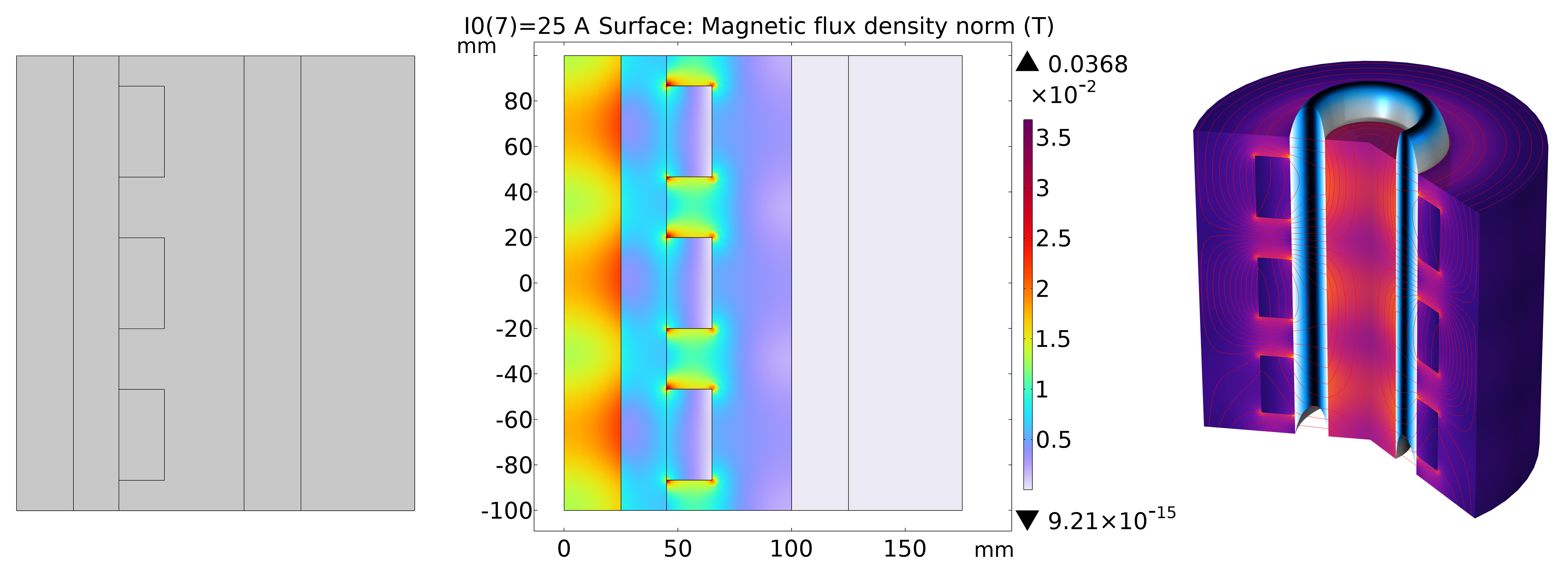
An axisymmetric magnetohydrodynamic pump. The geometry of the cross section (left), the magnetic flux density calculated on this cross section (middle), and the fluid velocity and magnetic field visualized in 3D (right).

Using a 2D Cross-Section Formulation

The 2D cross-section formulation is used when the geometry and physics are translationally invariant in one direction. In this case, a cross-sectional slice is taken perpendicular to this direction, which is defined as the out-of-plane z direction. The physics are solved on this 2D plane, with results given per meter of the out-of-plane length. The 2D solution can then be extruded to obtain the full 3D solution.

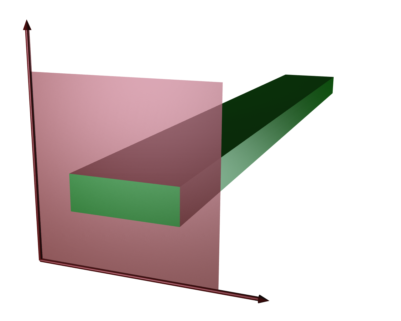
The modeling plane used in the 2D formulation (red) and its relationship to the full 3D geometry (green).

As in the 2D axisymmetric case, there are stricter requirements on the fluid flow than just being translationally invariant. The requirements to use a 2D cross-section model for MHD modeling are that:

• The geometry has to be translationally invariant in the z direction.
• The fluid flow has to be translationally invariant in the z direction and entirely in-plane.
• The magnetic and electric fields and the current have to be translationally invariant in the z direction. There is no restriction on their in-plane and out-of-plane components.

These requirements assume the geometry of the model to be infinitely long in the z direction. However, when the end effects are ignored and the length of the geometry is significantly longer in the z direction than in the x and y directions, the cross section of the model often provides sufficiently accurate results in the center of the system.

The requirement that the fluid flow is in-plane means that when modeling duct flow, a longitudinal slice through the duct can be used to generate a 2D model. However, it is not possible to take a slice through the duct in order to calculate the normal flow through the duct cross section.

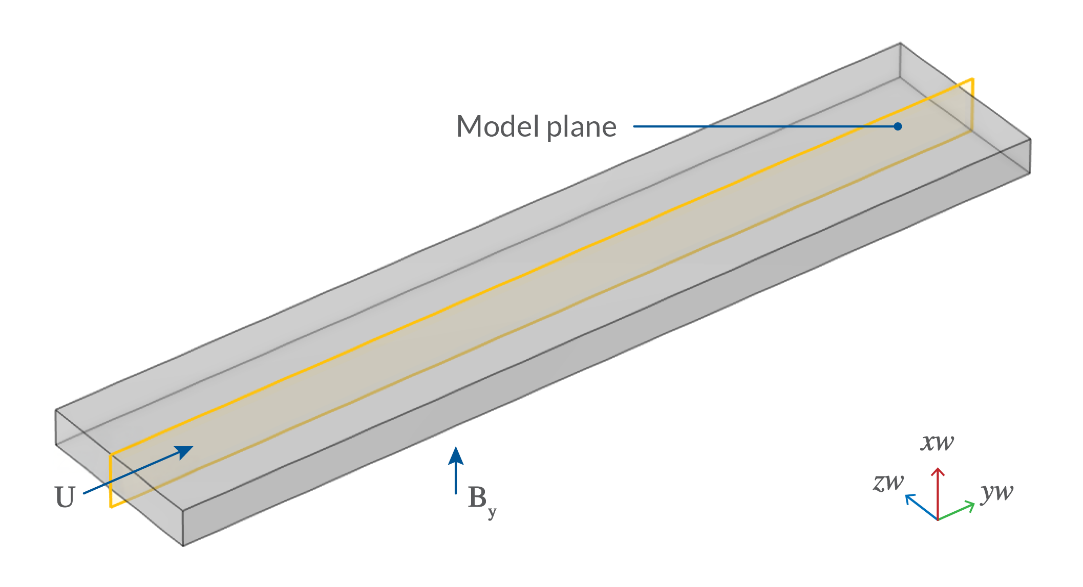
The 3D geometry and model plane used to create the 2D cross section for modeling flow between parallel plates.

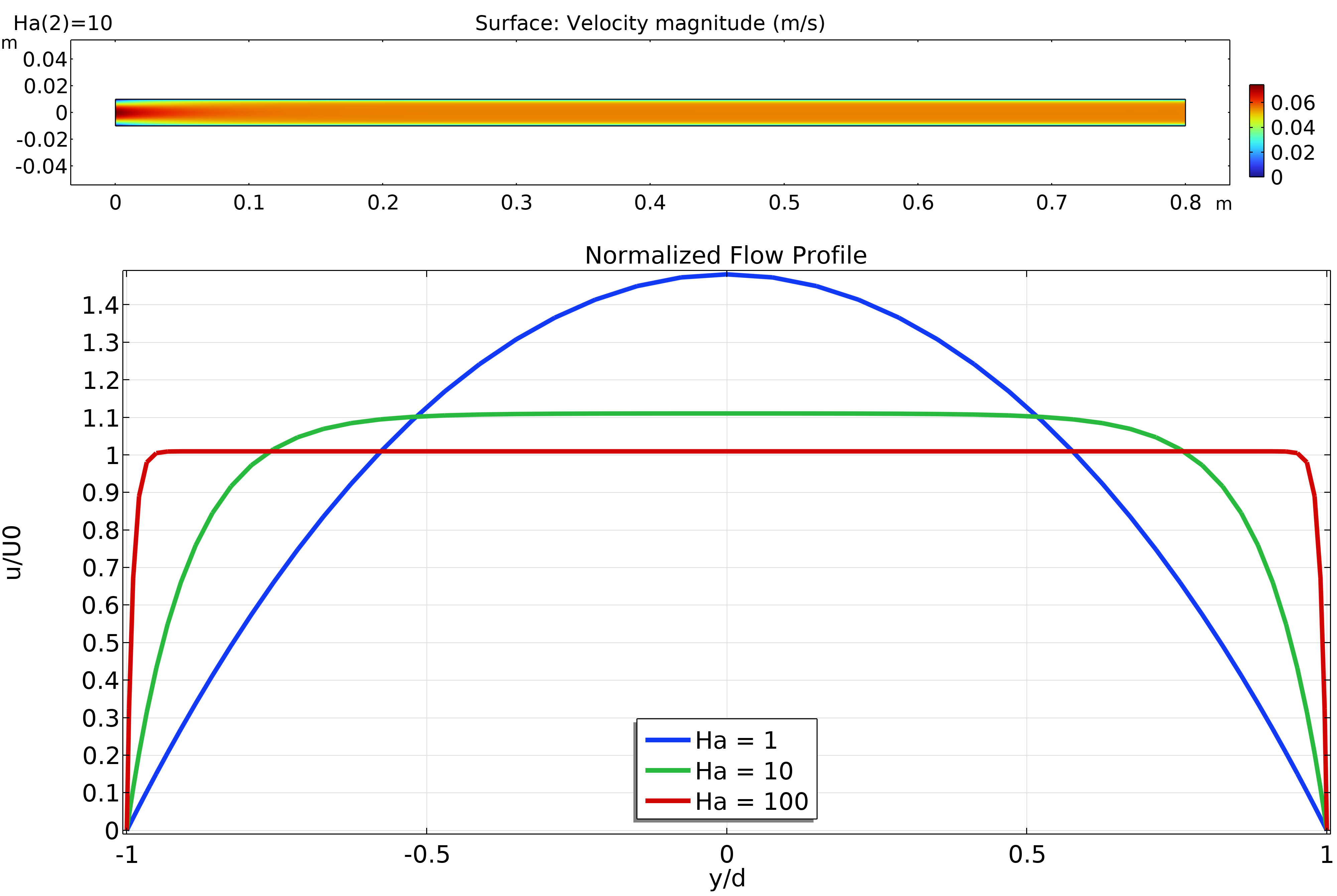
The calculated fluid velocity in the model plane (top). The profile of the fluid velocity plotted as a function of y for different Hartmann numbers (right).

Choosing the Electromagnetics Physics Interface

The Magnetohydrodynamics multiphysics coupling in COMSOL^® is compatible with several of the interfaces in the add-on AC/DC Module. These interfaces are:

• Magnetic Fields
• Magnetic and Electric Fields
• Rotating Machinery, Magnetic
• Magnetic Field Formulation

Out of these four interfaces, the two most commonly used interfaces for MHD modeling are the Magnetic Fields and Magnetic and Electric Fields interfaces. These two interfaces are separated by how they handle current conservation: The Magnetic and Electric Fields interface explicitly solves for a conserved current, while the Magnetic Fields interface assumes that all of the currents in the interface are already conserved. This difference affects when the interfaces can be used for MHD modeling.

The Magnetic Fields interface must only be used in a 2D or 2D axisymmetric formulation when all of the currents are in the out-of-plane direction.

The Magnetic and Electric Fields interface, as the most general electromagnetics interface, can be used for 3D models or 2D and 2D axisymmetric models with in-plane currents.

The other two interfaces, Rotating Machinery, Magnetic and Magnetic Field Formulation, are intended to be used for certain cases. The Rotating Machinery, Magnetic interface is designed for systems with moving mechanical components such as motors and generators. The Magnetic Field Formulation interface is designed for time-domain magnetic modeling of materials with strongly nonlinear E-J characteristics, such as superconductors. When these interfaces are combined with MHD modeling, they have the same current conservation limitations as the Magnetic Fields interface, meaning they can only be used for 2D and 2D axisymmetric models where all of the currents are in the out-of-plane direction.

Choosing the Fluid Flow Interface

The default assumption for MHD modeling is that it is being performed using the Laminar Flow interface to model the fluid flow. Even when the Reynolds number is large enough that it would otherwise indicate turbulent flow in the system, the Lorentz force can provide enough dampening in the system that it exhibits laminar flow or flow close enough to laminar that the laminar flow equations can be used. For this reason, it is recommended that the Laminar Flow interface is used as the interface for handling the fluid motion; and the Laminar Flow interface is the interface that is added to the system when the Magnetohydrodynamics, Out-of-Plane Currents or Magnetohydrodynamics, In-Plane Currents options are chosen from the Add Physics menu.

If it is essential to model turbulence in the fluid, the turbulence model type must be carefully considered. COMSOL^® offers three types of turbulent flow models:

1. Reynolds-averaged Navier–Stokes, eddy-viscosity models (RANS-EVM), where the time-averaged flow is calculated and the turbulent fluctuations averaged out
2. Reynolds-averaged Navier–Stokes, Reynolds-stress models (RANS-RSM), which still take the time-averaged flow but expand on the RSM-EVM models by explicitly calculating the components of the Reynolds stress tensor
3. Large eddy simulation (LES) models, where the largest eddies are directly modeled but the smallest eddies are filtered out of the equations

Our article "Basics of Modeling Turbulent Flow in COMSOL Multiphysics"offers more information on the individual turbulent flow models provided in the RANS-EVM and LES classes of turbulent flow models.

The Magnetohydrodynamics coupling works by applying the Lorentz force, , as a volume force within the fluid interface. Applying a volume force to the fluid is possible in all the RANS and LES turbulence interfaces, so you can select from those options for the fluid flow interface in the _ Magnetohydrodynamics_ multiphysics coupling. However, some care has to be taken to ensure that the volume force is consistent with any assumptions made by the different classes of turbulence models.

RANS-EVM models assume that the turbulence and eddies are isotropic in the fluid. As the Lorentz force acts in a single predominant direction — perpendicular to the current and magnetic field — this acts to dampen the flow and turbulence only in that direction. The isotropic turbulence assumption is thus broken. For this reason, RANS-EVM turbulence models should not be used in magnetohydrodynamics calculations.

The expansion of RANS-RSM to explicitly calculate the stress tensor means that these models can include anisotropic turbulence. COMSOL^® includes two RANS-RSM models: the Wilcox R-ω model and the SSG–LRR (Speziale–Sarkar–Gatsk/Launder–Reece–Rodi) model. These are designed for general hydrodynamic modeling rather than MHD modeling specifically. The general practice in turbulent MHD modeling is to use RANS-RSM models that have been developed explicitly to handle MHD flows.

LES models do not make assumptions about the anisotropy or isotropy of the turbulence, so while they can be used to model MHD, they are more computationally expensive and cannot be used in stationary simulations.

In this introductory course, only flow calculated using the Laminar Flow interface will be considered.

Summary

To summarize the decision-making process discussed here, refer to the flowchart shown below, which identifies whether a 2D, 2D axisymmetric, or 3D component is required for your model and which electromagnetics interface is recommended. While we have discussed a few different interfaces, the flowchart focuses on the Magnetic Fields and Magnetic and Electric Fields interfaces. The fluid flow interface used in this course will always be the Laminar Flow interface and thus will be used with the recommended component and electromagnetics interface.

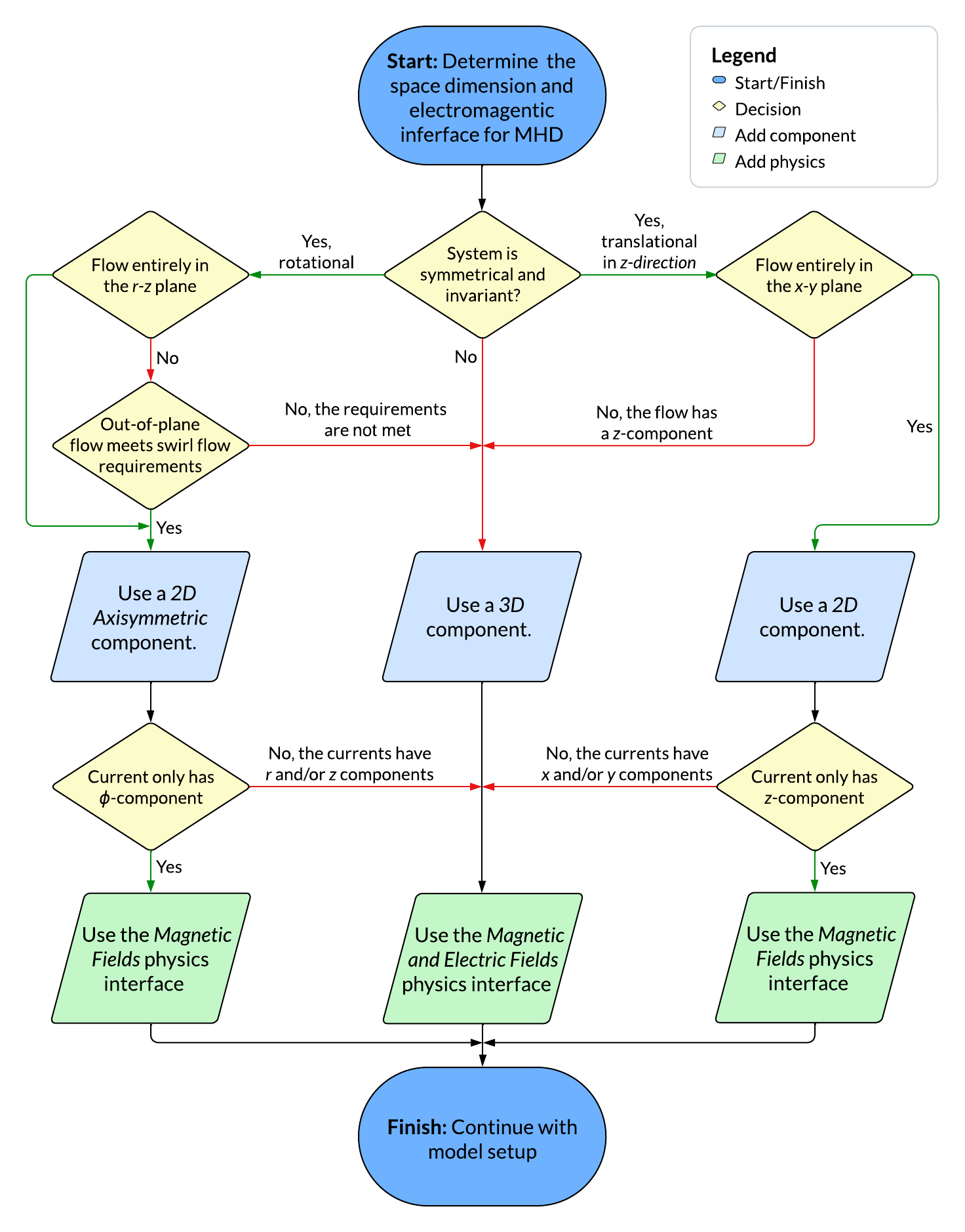
Flowchart summarizing the process of identifying a space dimension for an MHD model and the physics interfaces needed.

Further Learning

More information on the electromagnetic physics equations used in the Magnetic Fields and Magnetic and Electric Fields interfaces can be found here:

• The AC/DC Module User's Guide pages 38–59 and 86–94 of the PDF
• The Electromagnetics section of the Multiphysics Cylcopedia