More on Hyperparameters for Gaussian Processes
Following the discussion on Gaussian Process (GP) surrogate models from Part 5, here we give an introduction to the theory of hyperparameters for covariance functions used in GP surrogate models.
Covariance Functions and Hyperparameters
Let's now look at how closely the Gaussian process mean function (or GP surrogate model), resulting from the regression, approximates the function  , again based on only six data points. The figure below plots the GP mean function, as well as the six training points, in black, and the original function in magenta.

The original function in black and the GP prediction in magenta for a length scale  .
.
In this case, the covariance function used is a squared exponential (SE) kernel:

with signal variance  and correlation length, or length scale, .
The SE kernel is defined by two hyperparameters the signal variance,  , and the correlation length,
  . The signal variance controls the vertical variation (scale) of the function, while the correlation length determines the horizontal scale over which points are correlated. These hyperparameters influence the overall behavior and smoothness of the regression fit. There is also an additional possible hyperparameter in GP regression called the noise level variance,
  . When basing GP regression on computed data, the noise level variance can be set to a low value. It typically needs to be nonzero to avoid numerical instabilities during the Cholesky factorization performed as part of the underlying algorithm. Note that in the literature, the collection of hyperparameters for a surrogate model is commonly referred to as
  .
.
Varying the Length Scale
What happens if we use a different length scale? The results of using  and
and  are shown in the figure below. The fit is clearly worse in these cases.

The original function in black and the GP prediction in magenta for a length scale and signal variance .

The original function in black and the GP prediction in magenta for a length scale and signal variance .
After a bit of trial and error, we find that  gives a very good fit, as seen in the figure below, where the two curves are barely distinguishable. When using the built-in GP surrogate model in COMSOL Multiphysics®, this process of finding the length scale is automatic, as discussed later in this article.

The original function in black and the GP prediction in magenta for a length scale and signal variance .
Intuitively, a small value of the length scale "softens" the mean function and allows it to have more rapid variations, whereas a large value "stiffens" the mean function and gives it a tendency to vary more slowly.
Using an inappropriate length scale can lead to several issues that affect the quality of the fit.
When the length scale is too low, the GP model may:
- Overfit data with very fine details, fitting even the noise. This results in overfitting, where the model captures noise rather than the underlying trend, leading to poor generalization on new data.
- Assume that data points are only correlated over very short distances. This can result in high predictive variance (uncertainty) between data points, especially in regions with sparse data, leading to less reliable predictions.
- Produce highly oscillatory predictions that do not reflect the true underlying process, particularly in smooth or continuous data.
When the length scale is too high, the GP model may:
- Fit the data with excessive smoothness, failing to capture important variations and details in the data. This results in underfitting, where the model is too simplistic and does not adequately represent the true signal. An overly smooth model may fail to adapt to the local structure of the data, resulting in poor generalization and inaccurate predictions for new data points.
- Assume that data points are correlated over large distances, leading to overly confident (low variance) predictions even in regions with sparse data. This can misrepresent the uncertainty of the predictions.
Varying the Signal Variance
Let's now see what happens if we we keep and now vary the signal variance. The figures below show the result of using  ,
,  , and
, and  , respectively.

The original function in black and the GP prediction in magenta for a length scale and signal variance  .
.

The original function in black and the GP prediction in magenta for a length scale and signal variance  .
.

The original function in black and the GP prediction in magenta for a length scale and signal variance  .
.
We see that the value gives virtually as good of a fit as . Note that the GP mean function does not necessarily interpolate the input data exactly. For small values of the signal variance, the regression assigns relatively less importance to the training data (known values).
There is a point of diminishing returns where increasing the signal variance further does not significantly improve the fit. This is because the primary role of the signal variance is to scale the output, and once it reaches a level where it can adequately capture the variance in the data, increasing it further will not provide additional benefit.
Note that we should not use an unnecessarily large value for the signal variance. When the signal variance is too large, the GP model may:
- Become excessively flexible, allowing it to fit the noise in the training data rather than the underlying trend. This results in overfitting, where the model captures random fluctuations in the data rather than the true signal, leading to poor generalization on new data.
- Produce overly confident predictions (low predictive uncertainty) even in regions with sparse data. This can mislead the interpretation of the model's confidence in its predictions.
- Exhibit numerical instability in the inversion of the covariance matrix. This can lead to problems in computing the predictions and the associated uncertainties, making the model unreliable.
- Exhibit unrealistic oscillations or extreme values in the predicted function, especially in regions where data points are sparse. This can make the model's predictions physically or logically implausible.
Note that COMSOL Multiphysics® will automatically find an optimal signal variance, as explained further below.
Extrapolation
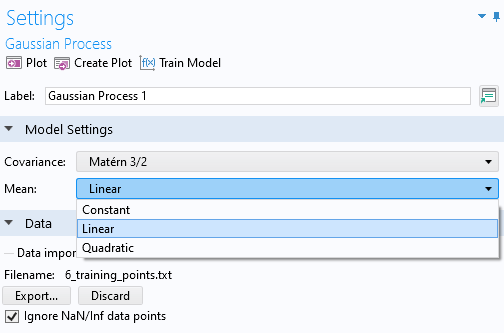
A GP model should preferably not be used for extrapolation. However, if you need to control the extrapolation behavior, you can change the Mean option in the Gaussian Process function Settings window, as shown in the figure below.
 Part of the Settings window for the Gaussian Process function, with the options for the Covariance setting expanded and shown.
The different mean options in the Gaussian Process function Settings window.
The default setting is Constant but you can change this to Linear or Quadratic. Plots of a GP surrogate model based on the six data points from the previous example, with the Mean setting set to Constant and Linear, are shown in the figures below, respectively. In this case, the Quadratic option is not a good choice since the data does not exhibit a quadratic type of behavior. In the Constant case, outside of the domain of definition of the training data, the GP function will return to a mean value, which is calculated directly from the training data. For the Linear and Quadratic options, polynomial terms are added to the prior distribution, and their coefficients are computed as part of the regression. A similar regression procedure is shown, for the linear case, in the blog post on Using Radial Basis Functions for Surface Interpolation.

A GP surrogate model with a constant mean function.

A GP surrogate model with a linear mean function.
Note that in the case of a Constant mean, if the training data has large gaps, the GP function will return to the mean value computed from the training data, as shown in the figure below where the data points from the previous example have been divided into two groups and separated by a large distance. This happens because the covariance function has a certain correlation length, determined through hyperparameter optimization, and the influence of points that are far apart diminishes exponentially as their distance grows.

A GP surrogate model with a constant mean function with large gaps in the data.
Hyperparameter Optimization and Adaptive GP Regression
In COMSOL Multiphysics®, the hyperparameters are automatically adjusted using an optimization algorithm, and, as a user, you never need to adjust the signal variance or length scale. What about cases where we have multiple outputs (quantities of interest)? How are the hyperparameters handled? A GP surrogate model with multiple outputs corresponds to a series of GP regression models, one for each output. The hyperparameters for these models are optimized individually for each regression model.
The hyperparameter optimization algorithm finds the hyperparameter values that make the observed data most probable under the assumed GP model. The algorithm is based on a global maximum likelihood optimization method. Since the log-likelihood expression used may have multiple local optima, the local optimizer for training the hyperparameters is started repeatedly by specifying different starting points in the hyperparameter space. By default, the number of restart points for training the hyperparameters is automatically chosen such that they are in the regions where the hyperparameters render relatively small negative log-likelihood.
When using adaptive GPs in the Uncertainty Quantification Module, the GP model is constructed adaptively by adding a new input parameter point at the location of the maximum entropy — when used for sensitivity analysis or uncertainty propagation. When the GP model is used for reliability analysis, the location of the maximum expected feasibility function is used instead.
In this context, the standard deviation of the GP model is used as the measure of entropy. For reliability analysis, the GP is trained to accurately approximate the underlying model primarily in regions that satisfy reliability conditions. The maximum expected feasibility function is used to identify adaptation points.
To explore the input parameter space and exploit the latest GP model, a global optimization problem is solved at each adaptation step to find the location corresponding to either maximum entropy or maximum expected feasibility function. There are two types of global optimization methods: the Dividing Rectangles (DIRECT) method and the Monte Carlo method, with the DIRECT method being the default choice.
For nonadaptive GPs, this global optimization procedure is used to determine the maximum entropy as an error estimation of the model. Note that nonadaptive GP models are not used for reliability analysis. Adaptive GP models, on the other hand, require a sufficient number of initial model evaluations to locate “good” adaptation points, which improve the accuracy of the GP model. An initial dataset with too few sample points can hinder the exploration of unsearched regions. This issue can be addressed using the Improve and analyze option to append more samples via sequential optimal Latin Hypercube Sampling (LHS), ensuring the samples randomly fill the entire input parameter space.
It is also important to note that for adaptive GPs built on input parameters with long tails (near-zero lower CDF, or cumulative distribution function, and near-one upper CDF), most initial sample points will be located in regions where input parameters have high probability. Consequently, the accuracy of the GP model in regions with low probability will be lower due to the lack of sample points, and most adaptation points will likely be placed in these low probability regions. To create a GP model with high accuracy across the entire input-parameter space under these circumstances, it is recommended to use a uniform distribution based on the minimum and maximum values corresponding to the lower and upper CDFs.
Training and Validation Settings
The settings for hyperparameter optimization as well as for validation are located in the Training and Validation section in the Gaussian Process function Settings window, as shown below.

The Training and Validation section for the GP surrogate model.
The following table summarizes these settings.
| Setting | Values | Description |
|---|---|---|
| Method for number of restart points | Automatic or Manual | The Automatic method uses 2*m+4 restart points, where m is the number of input parameters (surrogate model dimension). |
| Number of restart points for training | Positive integer | This specifies the number of restart points used by the global hyperparameter optimization algorithm. |
| Optimization method for error estimation | Direct or Monte Carlo | This setting specifies the method used for surrogate model error estimation, which is computed after the hyperparameter optimization is finalized. The Direct method uses a recursive subdivision algorithm to find the maximum surrogate model error by varying the input parameters. The Monte Carlo method uses a user-defined number of randomly distributed input parameters. |
| Maximum surrogate evaluations for optimization | Nonnegative integer | This setting applies to the Direct method and limits the number of surrogate model evaluations during surrogate model error estimation. |
| Maximum number of optimization iterations | Nonnegative integer | This setting applies to the Direct method and limits the total number of iterations during surrogate model error estimation. |
| Surrogate evaluations for optimization | Nonnegative integer | This setting applies to the Monte Carlo method and limits the number of surrogate model evaluations during surrogate model error estimation. In other words, this number specifies the number of random evaluation points. |
| Maximum matrix size | Integer greater than 1 | This setting limits the size of the covariance matrix that is inverted during the training process. The default value is 2000. |
| Random seed type | Fixed or Current computer time | This setting determines the type of random seed used for the random process to sample in the input parameter space. |
| Random seed | Integer | This setting applies to the Fixed method for defining the random seed and specifies a user-defined seed value. |
| Validation data | None, Random sample of data values, Every Nth data value, Last part of data values, Separate table | This setting specifies the method used for selecting the validation data. The validation data is a portion of the training data set aside for validation purposes. |
Iterations and Settings for Uncertainty Quantification and GP Training
Note that when performing an Uncertainty Quantification study that utilizes a GP surrogate model, there are multiple levels of iterations that take place, for example, for the uncertainty propagation study type. The iterations and termination criteria are as follows:
- Outer Loop: Uncertainty Quantification study
- Controlled By:
- Surrogate model (GP or Adaptive GP)
- GP
- Terminate when Number of input points are reached
- Adaptive GP
- Controlled By:
- Relative tolerance
- Initial number of input points
- Maximum number of input points
- Iteration:
- Terminate when Relative tolerance is met or input points reach Maximum number of input points
- Controlled By:
- Controlled By:
- Next Level: Global GP Hyperparameter Optimization with Subsequent Global Error Estimation
- Global Hyperparameter Optimization Iteration:
- Loop over each restart point
- Controlled By:
- Number of restart points for training
- Once the best global GP hyperparameters are found, the GP error is estimated through a separate global optimization algorithm
- Global Error Estimation Iteration:
- Controlled By:
- Optimization method (Direct or Monte Carlo)
- Direct Method:
- Iteratively find the maximum surrogate model error by varying the input parameters through a recursive subdivision algorithm
- Terminate when iterations reach Maximum number of optimization iterations or surrogate evaluations reach Maximum surrogate evaluations for optimization
- Monte Carlo Method:
- Evaluate surrogate model error for random input parameters
- Terminate when evaluations reach the number Maximum surrogate evaluations for optimization
- Controlled By:
- Global Hyperparameter Optimization Iteration:
- Innermost Level: GP Hyperparameter Optimization
- Controlled By:
- Derivative-free constrained optimizer
- Iteration:
- Terminate when a relative tolerance is met or a number of max log-likelihood evaluation is reached (these values are fixed and cannot be changed by the user)
- Controlled By:
 A screenshot of UI with the Uncertainty Quantification study selected in the Model Builder and the corresponding Settings window shown.
Some of the settings for the Uncertainty Quantification study used in Part 4 of the introductory course on UQ. Here an adaptive GP is used.
The final GP error estimation is only done once for the best GP model found from the global GP hyperparameter optimization. This error estimation is output to the Information section of the Settings window and computes the maximum GP standard deviation and normalizes with the population standard deviation from the input data.
When training a GP surrogate model without uncertainty quantification, only the Next Level and Innermost Level are run.
When the computation is complete and the maximum number of iterations or input points is reached without meeting the relative tolerance value, a warning is displayed in the Log window, and a warning icon appears in the model tree under the Job Configuration > Uncertainty Quantification node as shown below.
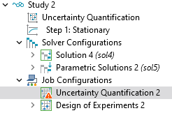 A close-up of part of the model tree, under the Study node, with the Job Configurations node expanded and the Uncertainty Quantification subnode, which displays a white exclamation point contained in an orange triangle on the node's icon, selected.
The warning indicator shows that the relative tolerance criterion was not met.
In most cases, the most effective way to increase the accuracy of the surrogate model is to increase the number of input points. However, this will require additional finite element model solves, leading to longer computation times.
Submit feedback about this page or contact support here.