Learning Center

Course:

Modeling Speaker Drivers in COMSOL Multiphysics^®

BACK TO LEARNING CENTER

Modeling Speaker Drivers – Lumped Methods

The first four parts of this course discussed how to perform a full electro-vibroacoustic analysis of a speaker driver using the finite element method. Such a detailed analysis including all of the acting electromagnetic and mechanical components of the driver is necessary at the stage of designing the driver. When the analysis is at the system level — for example, to study the behavior of the driver in a mounting system or to design a waveguide for achieving a specific radiation pattern — including all driver components in the model and solving all of the included physics can be expensive and even not feasible. It is also not necessary when a lumped representation of the driver is available and applicable.

A lumped model is applicable when the different mechanical components in the driver have the piston-like motion, which is a good assumption for lower frequencies when the dimension of the driver is much smaller than the wavelength. It is possible to use the following lumped methods to represent the behavior of the driver based on the information available at hand:

Prescribing a motion on radiating surfaces. This should be used when you have the exact information on the moving surfaces that radiate sound. The quantity characterizing the movement can be either displacement, velocity, or acceleration. In this approach there is no feedback from the acoustic domain to the transducer, and the source impedance is not included.
Using a lumped representation of the electromagnetic force to drive the speaker. Assuming a moving coil transducer, the Lorentz force acting on the voice coil is calculated using lumped parameters that include the force factor of the voice coil and its blocked coil impedance (i.e., the electric impedance when the coil is at standstill).
Using a lumped electromechanical (or electroacoustic) representation of the driver that is characterized with the small-signal parameters for small deformations (the so-called Thiele–Small parameters) or large-signal parameters for large deformations. This lumped electrical circuit analogy represents the behavior of both the electrical and mechanical speaker components, allowing a two-way coupling between the transducer and the acoustic domain.
Using an electrical circuit analogy for the electrical system and a lumped mechanical analogy for the mechanical system with lumped components such as masses, springs, and dampers.

The parameters used in all four of these methods can be obtained either from measurements or solved submodels, and they can be functions of frequencies. The first two methods do not solve the electromagnetic (EM) field at all, whereas the last two do include the electrical property in the computation, but it is solved by 0D ordinary differential equations (ODEs). All of these lumped models can be coupled to a finite element model that solves the acoustic field. Let's take a closer look at these four methods.

Method One: Prescribing the Movements of Radiating Surfaces

To use this method, you need the data that directly describe the movement of radiating surfaces (e.g., the motion of the moving diaphragm) or the output from the speaker (e.g., the acoustic output at a specific surface), and you usually only need to include the radiating surfaces in the geometry to represent the driver. Very often, a single pressure acoustics model is solved, and the radiating surfaces are either interior boundaries (when the acoustic fields on both sides are solved) or exterior boundaries (when sound radiation to only one side is modeled) of the simulated acoustic domains. Examples of this include the following tutorials:

The images below show the boundaries (highlighted in blue) representing the radiating surfaces in these examples.

Four images of acoustic devices with a surface selected in blue.
The boundaries highlighted in blue represent the radiating surfaces of speaker drivers in the tutorials.

The following images show how the movements are prescribed at the radiating surfaces. You can specify acceleration, velocity, or displacement in the normal direction or their components on both interior and exterior boundaries. Again, these quantities can be frequency dependent if applicable. The prescribed movement can also be a function of spatial coordinates or a solution from a solved submodel.

Settings for Interior Normal Velocity are shown along with a graphic of a 2D model with red arrows tangential to boundaries selected in blue.
An Interior Normal Velocity boundary condition is added to prescribe the movement at internal radiating surfaces.

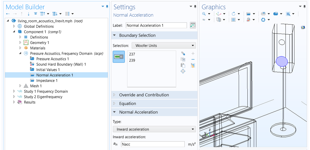Settings for Normal Acceleration are shown with a graphic of a wireframe box with a blue circle on the leading face.
The movement at external radiating surfaces is prescribed with an applied Normal Acceleration boundary condition.

Please note that this method uses an idealized source where there is no acoustic feedback to the source. However, it can still be a valuable analysis approach, especially when you are mostly interested in the radiation characteristics or the spatial response.

Method Two: Using the Lumped Electromagnetic Force

Base on the Lorentz force law, the total net force exerted on a current-carrying wire placed in a magnetic field and the back EMF (the induced voltage in the moving coil) are calculated by the following equations:

where is the force vector, is the length of the coil, is the total current in the coil, is the externally generated magnetic flux density, is the applied driving voltage, denotes the back EMF, is the blocked electric impedance, and is the velocity vector of the moving coil.

From these relations we can obtain the following lumped representation of the total driving force on the voice coil in a dynamic driver like the one described in Part 2 of this series:

where is the product of the magnetic field strength and the voice coil length and is called the force factor. is the coil velocity in the axial direction.

The force factor and the blocked electric impedance can be obtained from measurements or calculated from a detailed FEM model as described in Part 2. We will discuss how to calculate them in Part 6.

With known and for a specific driver in use, the total force experienced by the coil can be specified using the above expression. This method requires including the moving parts of the driver in the geometry and running a full vibroacoustic (acoustic–structure interaction) analysis to model the vibrations of the moving parts and the sound radiating from them. Examples using this approach include the following tutorials:

Let's take a look at the first example, which models the acoustic behavior of a loudspeaker driver mounted in a bass reflex (vented) enclosure. The electromagnetic properties of the driver are supplied from the Loudspeaker Driver — Frequency Domain Analysis tutorial model. Different structural components of the loudspeaker are modeled with the Solid Mechanics and Shells interfaces, such as the enclosure and driver. The acoustic cavity within the enclosure is modeled with the Pressure Acoustics, Frequency Domain interface, while the Pressure Acoustics, Boundary Elements_interface is used to model the infinite domain surrounding the enclosure. The _Acoustic-Structure Boundary multiphysics coupling is used to connect the different acoustic and structural physics, and the Acoustic BEM-FEM Boundary multiphysics coupling is used to couple, at the vent, the interior acoustics with the exterior. An image of the geometry is shown below. The speaker driver is oriented in the -x direction, and only half of the geometry is modeled using symmetry condition at the y = 0 plane.

One symmetric half of a gray box with an extruded cylinder and cone.
The geometry used in the Loudspeaker Driver in a Vented Enclosure tutorial.

In this example, is a parameter with a constant value of 10.48 N/A (Global Definitions > Parameters 1 node). is a variable defined by a complex-valued function of the frequency (Component 1 > Definitions > Variables 1 node). and are taken from the Loudspeaker Driver — Frequency Domain Analysis tutorial. In Study 1 of the tutorial, a small-signal analysis of the magnetic field is completed assuming the coil is fixed. This allows the force factor and the frequency-dependent blocked coil parameters to be calculated, including the coil impedance, coil resistance, coil inductance, etc. The coil resistance, , and the coil inductance, , are then exported and saved in two .txt files. We will discuss in detail how to run such an analysis in order to extract these parameters in Part 6.

The two .txt files are imported into the Loudspeaker Driver in a Vented Enclosure model using two interpolation functions (Interpolation 1 (Rb) and Interpolation 2 (Lb) under Component 1 > Definitions). The image below shows how these two functions are used to define the blocked coil impedance, , which is in turn used to define the driving force, .

A_Variables Settings window showing the variables for the total driving force in the model.
The total driving force defined in the model.

The force is then applied as opposing forces acting over the voice coil and the soft irons (the top plate and pole piece) in opposite directions in the Solid Mechanics interface, as seen in the image below. In the model, the total applied force on the entire coil, , is multiplied with a factor of 0.5 as one symmetry is in use and only half of the coil is modeled. Here, the magnetic system is not assumed to be fixed, so the reaction force is applied to include the effect of its movement. However, the reaction force on the magnetic circuit only has a minor influence on the response, as the magnet system is much heavier than the coil and speaker cone.

Two identical wireframe cone-shaped objects are shown with different solid blue areas highlighted in the narrow section.
The lumped electromagnetic force is applied as opposing forces acting over the voice coil and the magnet system in opposite directions.

The acoustic–structure interaction model can be solved using a single Frequency Domain study step.

Method Three: Using a Lumped Circuit Model

Electric circuit representations of transducers are well known and widely used in the loudspeaker industry. The parameters that characterize the low-frequency performance of a speaker driver are commonly known as the Thiele–Small or the small-signal parameters for small deformations or the large-signal parameters for large deformations. The former case can be solved using a frequency-domain analysis because the problem stays linear. The Thiele–Small parameters are constant in regard to coil displacement although they can be functions of frequencies. However, for the case of large deformations, a transient analysis is required because the lumped parameters are defined by functions of coil displacement and the problem becomes nonlinear.

You have the option to only lump the electrical components of the driver (similar to the method described earlier) and model the mechanical components fully, or apply the lumping to both. Either way, the lumped components are simulated using an Electrical Circuit interface, which can be coupled to an acoustic or acoustic–structure interaction FEM model to conduct a system analysis. Let's use the Lumped Loudspeaker Driver tutorial as an example to discuss the analogous circuit and circuit–FEM coupling using built-in features.

The driver modeled here is similar to the one used in Part 2. One notable distinction is that the mechanical and electrical components inside the dotted box (in the leftmost diagram below) are lumped and modeled using an Electrical Circuit interface. The electrical diagram includes the voice-coil and magnetic system (permanent magnet and pole pieces), and the mechanical diagram includes the moving mass of the voice coil and speaker cone, the spring effect of the spider and outer suspension, and the possible losses that will result from damping in these suspensions. The circuit diagrams below show the analogous circuits for the electrical and mechanical properties of the speaker driver.

A 2D diagram of labeled mechanical and electrical components and two circuit diagrams.
The components of the speaker driver inside the dotted box (left) are modeled by the analogous circuits for the electrical properties (upper right) and mechanical properties (lower right).

In the circuit for the electrical system, the external voltage source is denoted by , and the generator output resistance is . In this model, is set to zero. The voice coil resistance is , and the voice coil inductance is , which is frequency dependent. The losses in the magnetic circuit are modeled through the frequency-dependent resistance . The current controlled voltage source, , represents the back-induced electromagnetic voltage generated when the voice coil moves with velocity in the magnetic field . Here, is the force factor, the product of the magnetic field strength and the voice coil length . In the electrical circuit, the current is denoted as .

It is worth mentioning that many classical lumped representations exist for the voice coil impedance. What's used here is a version of the so-called Leach model. Other models can readily be set up, like a simple LR, the LR-2, the LR-3, or the so-called Wright model. The desired model topology is defined when setting up the Electrical Circuit interface.

In the circuit for the mechanical system, the impedance analogy is used. The current in the circuit, , is the velocity of the voice coil and speaker cone in the axial direction (see the left image in the above figure). The Lorentz force on the voice coil with current, , is given by . The force acts on a system of mass (voice coil and diaphragm assembly). The resistance, , models the damping and mechanical compliance, , in the speaker suspensions (both spider and outer suspension). Finally, the voltage source, , represents the pressure force acting on the speaker diaphragm (in the axial direction). Notice the minus sign that indicates that the force acts against the movement of the diaphragm. The pressure force is given by

where is the pressure drop across the diaphragm and is the axial component of the surface normal . This expression gives the couplings from the acoustic finite element model to the lumped circuit model. The coupling from the circuit model to the finite element model is the result of specifying the velocity, , on the surface of the diaphragm, which is given by

where is the unit vector in the axial direction and is the current in the mechanical circuit analog.

These expressions and couplings are automatically handled and set up with the various built-in Lumped Speaker Boundary conditions in COMSOL®. Let's look into them now.

Circuit–FEM Coupling Using Lumped Speaker Boundary Conditions

The computational domain where the pressure acoustics FEM model is solved is shown below. It represents the speaker (red line), including the cone, dust cap, and outer suspension, in an infinite baffle in a 2D axisymmetric model.

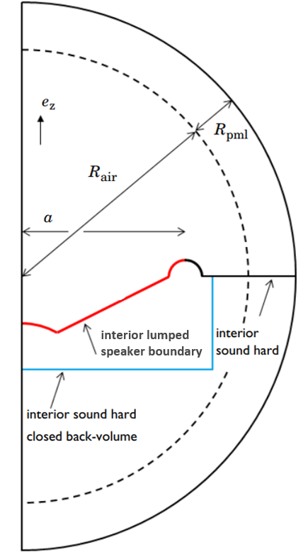A semicircle with labeled red, blue, and black lines on the interior.
Computational domain and boundary conditions for the FEM pressure acoustics model.

The coupling between the FEM pressure acoustics model and the lumped circuit model needs to be applied at the speaker boundaries. This coupling can be accomplished with the following two steps:

Add an Interior Lumped Speaker Boundary feature to the Pressure Acoustics, Frequency Domain interface, as shown in the image below. It takes the current from the mechanical circuit analog (i.e., in the circuit diagram or in the equation shown in the UI) and uses it to specify the axial velocity, , at the speaker surfaces. It also calculates the axial pressure force (i.e., in the circuit diagram or in the equation shown in the UI) induced by the pressure drop across the diaphragm, which in turn is fed back to the lumped circuit model.

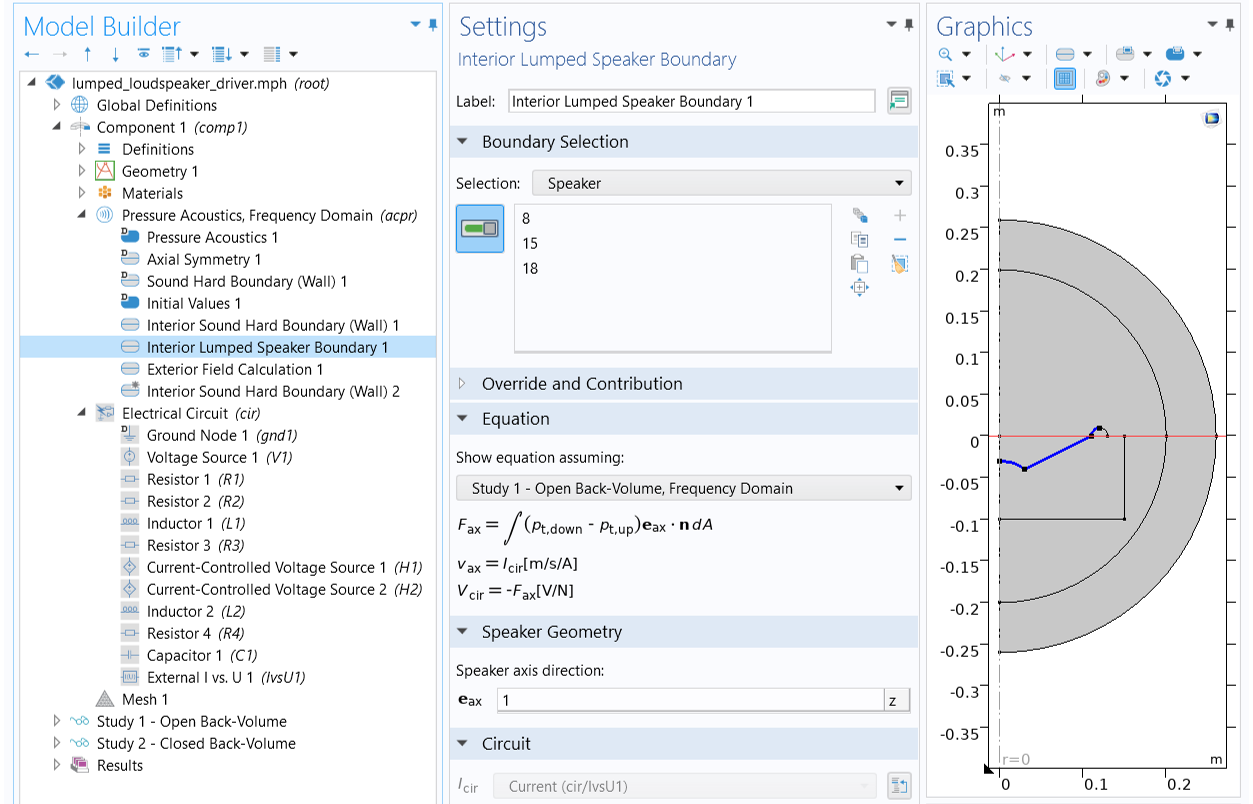A Settings window for an Interior Lumped Speaker Boundary feature and a gray semicircle with blue selected boundaries.
The FEM acoustic model is coupled to the lumped circuit driver model via the built-in Interior Lumped Speaker Boundary feature.

Add an External I vs. U feature to the Electrical Circuit interface and set the Electric potential to Voltage from lumped speaker boundary, as shown in the image below. This feature takes the axial pressure force calculated in the Interior Lumped Speaker Boundary feature in the Pressure Acoustics, Frequency Domain interface and applies it as a voltage source within the electrical circuit.

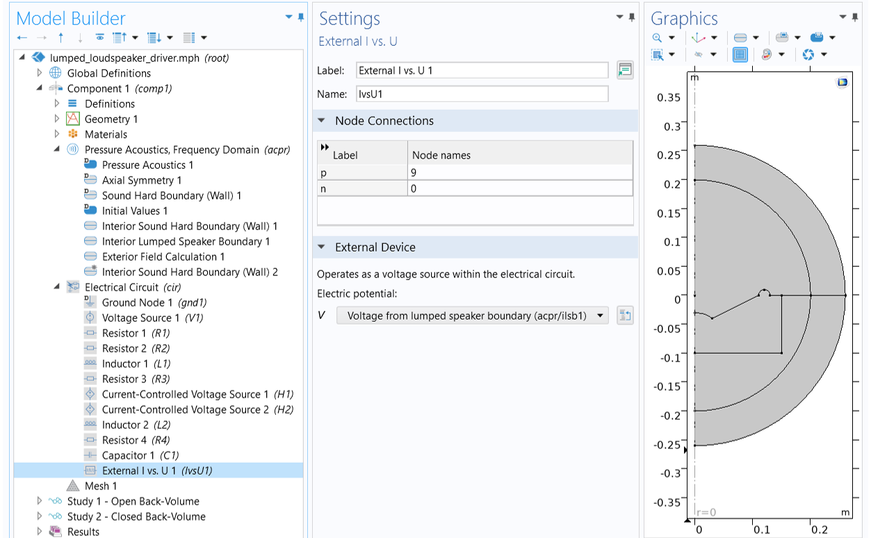A Settings window for an External I vs. U feature and a gray semicircle with black internal boundaries.
The lumped circuit model is coupled to the FEM acoustic model by an External I vs. U feature.

When the diaphragm is modeled with a solid and not an interior boundary/shell (interior condition) like the one discussed above, you can set up an interior lumped loudspeaker by adding two Lumped Loudspeaker Boundary features, one applied to the upper boundaries and the other to the lower boundaries, as shown in the image below. For previous versions (through version 6.1), it is necessary to set the back volume correction to a large value to remove the compliance of this lumped representation. In versions 6.2 and up there is a No correction option available that should be used, which gives zero correction impedance.

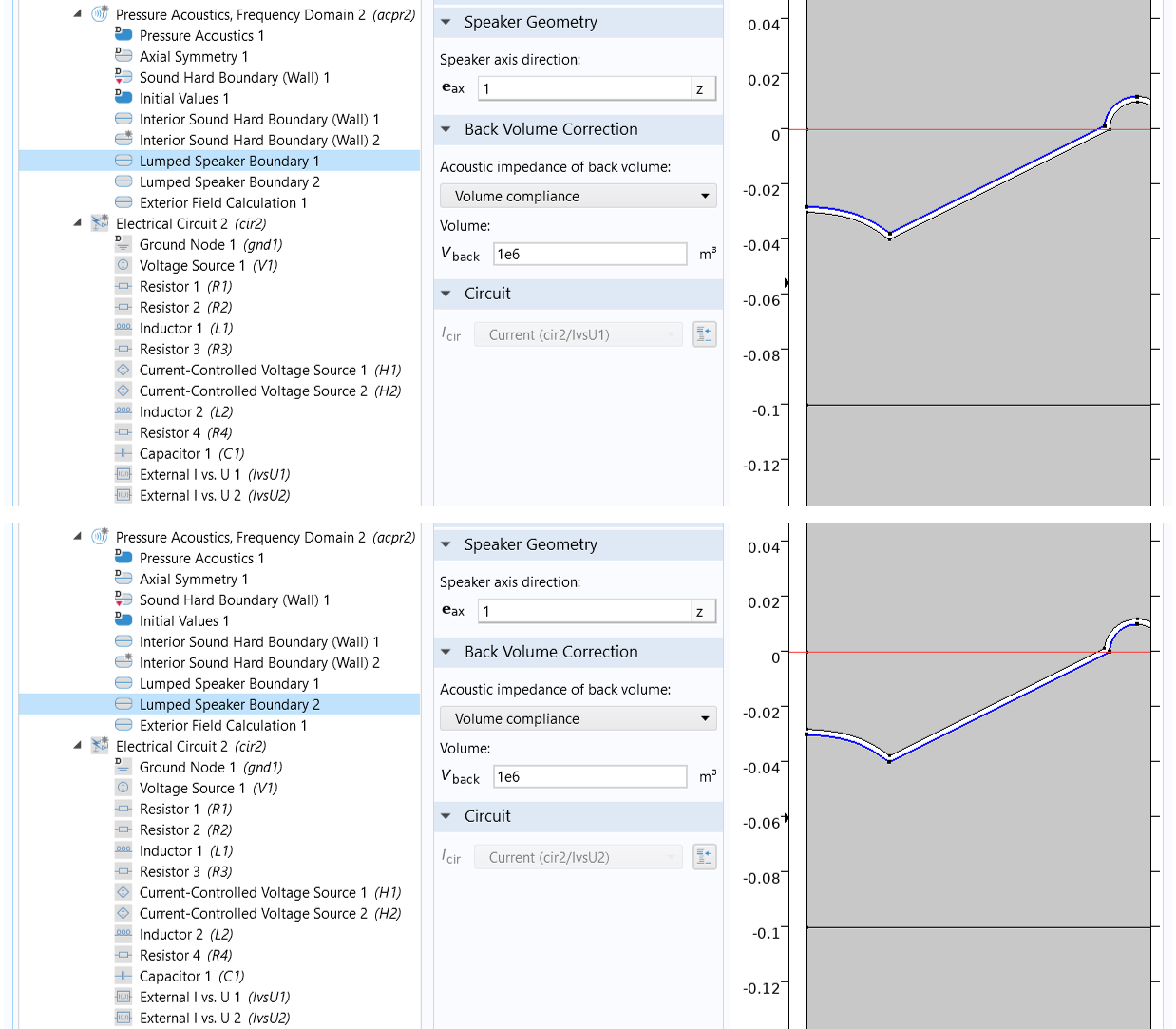Large back volume values are shown for two graphics with blue upper boundaries and blue lower boundaries, respectively.
A large value is set in the Back Volume Correction menu for a model built in version 6.1 or earlier.

The No correction option is selected in the Back Volume Correction menu for two Lumped Speaker Boundaries.
In versions 6.2 and up, use the No correction option, which sets correction impedance to zero.

Then, in the Electrical Circuit interface, two External I vs. U nodes should be added in series, as shown below. This version of the setup is demoed in Component 2 of the attached model (lumped_loudspeaker_driver_solid_diaphragm_62.mph).

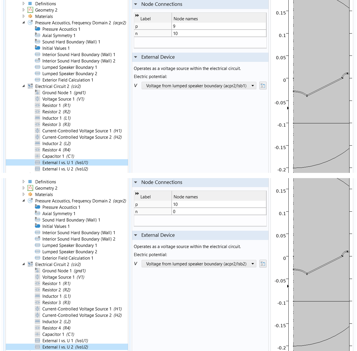A comparison of the Settings windows for the two External I vs. U nodes.
The circuit–FEM coupling setup when the diaphragm is modeled with a solid.

Using Lumped Speaker Boundary Features in a Transient Nonlinear Analysis

The Lumped Speaker Boundary features are also available in time-domain models where you can include large-signal parameters to simulate the nonlinear (large-signal) behavior of certain lumped components in a simplified loudspeaker analysis. Use of these features is showcased in the following tutorials:

These tutorials use the built-in coupling between the Interior Lumped Speaker Boundary feature and an equivalent electrical circuit for the mechanical and electrical system.

Let's look at the first example, where the model definitions are similar to the one we discussed in the previous section for frequency-domain analysis using Thiele–Small parameters. We now introduce a few large-signal parameters and solve a transient model to capture the nonlinear effects induced when the diaphragm undergoes large excursion. The large-signal compliance and force factor are nonlinear functions of the diaphragm's axial location, whereas the mechanical damping is a function of the diaphragm's axial velocity. These functions are defined as interpolation data and their time dependency arises from time-varying and . The axial position of the diaphragm is calculated and stored in a predefined global variable actd.ilsb1.x_ax, and the diaphragm's axial velocity is available through a predefined global variable actd.ilsb1.v_ax.

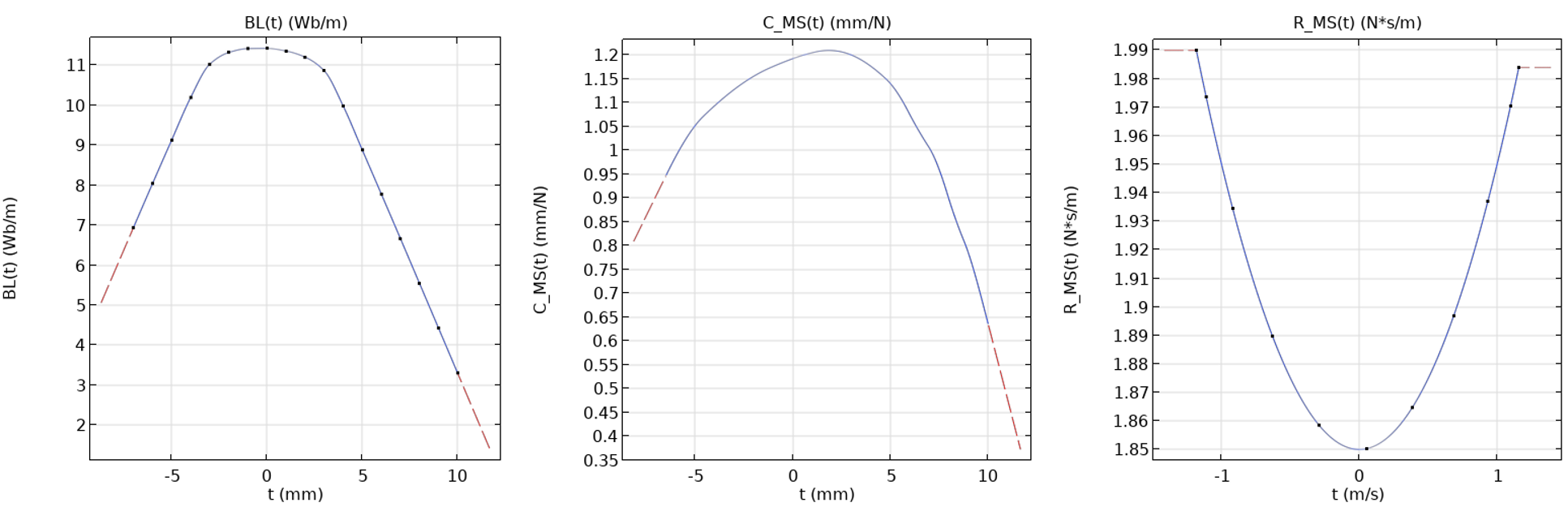Three 2D plots of signal compliance, force factor, and mechanical damping.
The interpolation function plots showing the dependency of the force factor, BL, and the compliance, C_MS, on the diaphragm's axial location (left and middle) as well as the relation between the mechanical damping, R_MS, and the diaphragm's axial velocity (right).

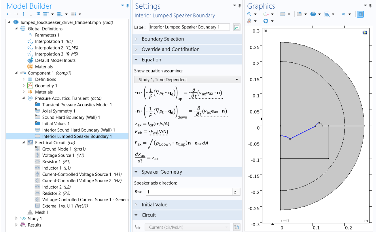A Settings window showing the equations for an Interior Lumped Speaker Boundary.
The diaphragm's axial location and axial velocity variables calculated in the transient Lumped Speaker Boundary feature.

Four Settings windows for H1, H2, R2, and G1 showing the equations used to define the large-signal parameters.
The calculated axial location and axial velocity used to define the large-signal parameters in the circuit model.

Note that in the frequency domain, the mechanical compliance is simply represented by a capacitor in the mechanical circuit. In the time domain, a capacitor device is not sufficient for describing the effect of a time-varying capacitance (whose time dependency is through ) because the built-in capacitor device uses the relation , which does not include the contribution from the time derivative of . The solution is to use a Voltage-Controlled Current Source device that has the current–voltage relation of so that the full time derivative is taken. The voltage of the device is stored in an internal variable named sens.v, which is ready for use to define the correct current–voltage relation.

The nonlinear effects associated with the compliance and force factor are especially important at lower frequencies. This is also where a lumped modeling approach has its main application. The image below shows the frequency spectrum of the nonlinear periodic part of the signal evaluated at a point 20 cm in front of the speaker, which is driven by a 50 Hz voltage source. This input signal will allow for the evaluation of the total harmonic distortion (THD); the signal can be modified to any desired signal, for example, if intermodulation distortion (IMD) is of interest.

A 2D line graph with labeled peak dB values at various frequencies.
The frequency spectrum of the acoustic signal evaluated at a point 20 cm in front of the speaker that is driven by a 50 Hz voltage source. Peak values shown for the generated harmonics.

Method Four: Using a Lumped Mechanical System Model

Here, we discuss another option for lumping the mechanical components. Although an electrical circuit representation (as described above) using the impedance analogy is commonly used, some users may prefer a lumped mechanical circuit using the mobility analogy. In that case, you can use a Lumped Mechanical System interface to model displacements and forces in the mechanical system with lumped components such as masses, springs, and dampers, while keeping an electrical circuit model for the electrical system. This is demonstrated in the Lumped Loudspeaker Driver Using a Lumped Mechanical System tutorial. As seen in the image below, the tutorial uses the same circuit model for the electrical components (upper right); however, a mass-spring-damper system is used to represent the driver's mechanical behavior (lower right).

A 2D diagram of a lumped mechanical system, a black circuit diagram, and a blue circuit diagram.
The components of the speaker driver inside the dotted box (left) are modeled by a lumped electrical circuit for the electrical properties (upper right) and a lumped mechanical system for the mechanical properties (lower right).

The mechanical system has the following components:

Mass ( ) representing the mass of voice coil and diaphragm assembly
Spring ( ) representing the stiffness of speaker suspensions (both spider and outer suspension)
Damping ( ) representing the possible losses in suspensions

Lumped Model–FEM Coupling

The lumped mechanical system needs to be coupled to the FEM pressure acoustics model as well as to the lumped electrical model. These couplings can be accomplished with the following three steps:

Add an Interior Normal Acceleration feature to the Pressure Acoustics, Frequency Domain interface and use the mass acceleration calculated in the Lumped Mechanical System interface to define the acceleration in the axial direction, as shown in the image below. The variable lms.M1_a saves the acceleration of Mass 1, M1, (corresponding to in the diagram) in the Lumped Mechanical System, lms, interface.

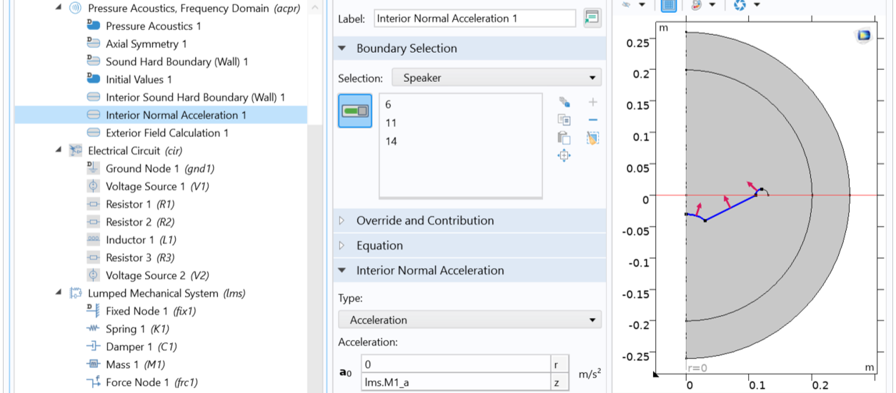An Interior Normal Acceleration feature Settings window and a semicircular graphic with red arrows tangent to the blue interior boundaries.
The mass acceleration from the lumped mechanical system is passed to the pressure acoustics model for sound radiation.

Add a Voltage Source node to the Electrical Circuit interface and use BL*lms.M1_v to define the voltage. The variable lms.M1_v saves the velocity of Mass 1 in the Lumped MechanicalSystem interface. This voltage source corresponds to in the lumped electrical circuit diagram, representing the back-induced voltage generated by the coil movement.

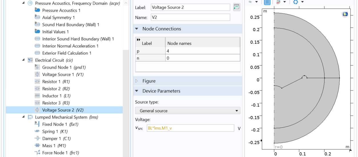A Voltage Source feature Settings window with voltage defined by an equation and a gray semicircular graphic.
The mass velocity from the Lumped Mechanical System interface is passed to the Electrical Circuit interface to include the back EMF.

Add a Force Node in the Lumped Mechanical System interface to include the Lorentz force, BL*cir.R2_i, acting in the axial direction, and the pressure force F_D. The variable cir.R2_i saves the coil current from the Resistor 2 node, R2, in the Electrical Circuit, cir, interface. F_D is the axial pressure force defined manually in the Model variables node (bottom image below).

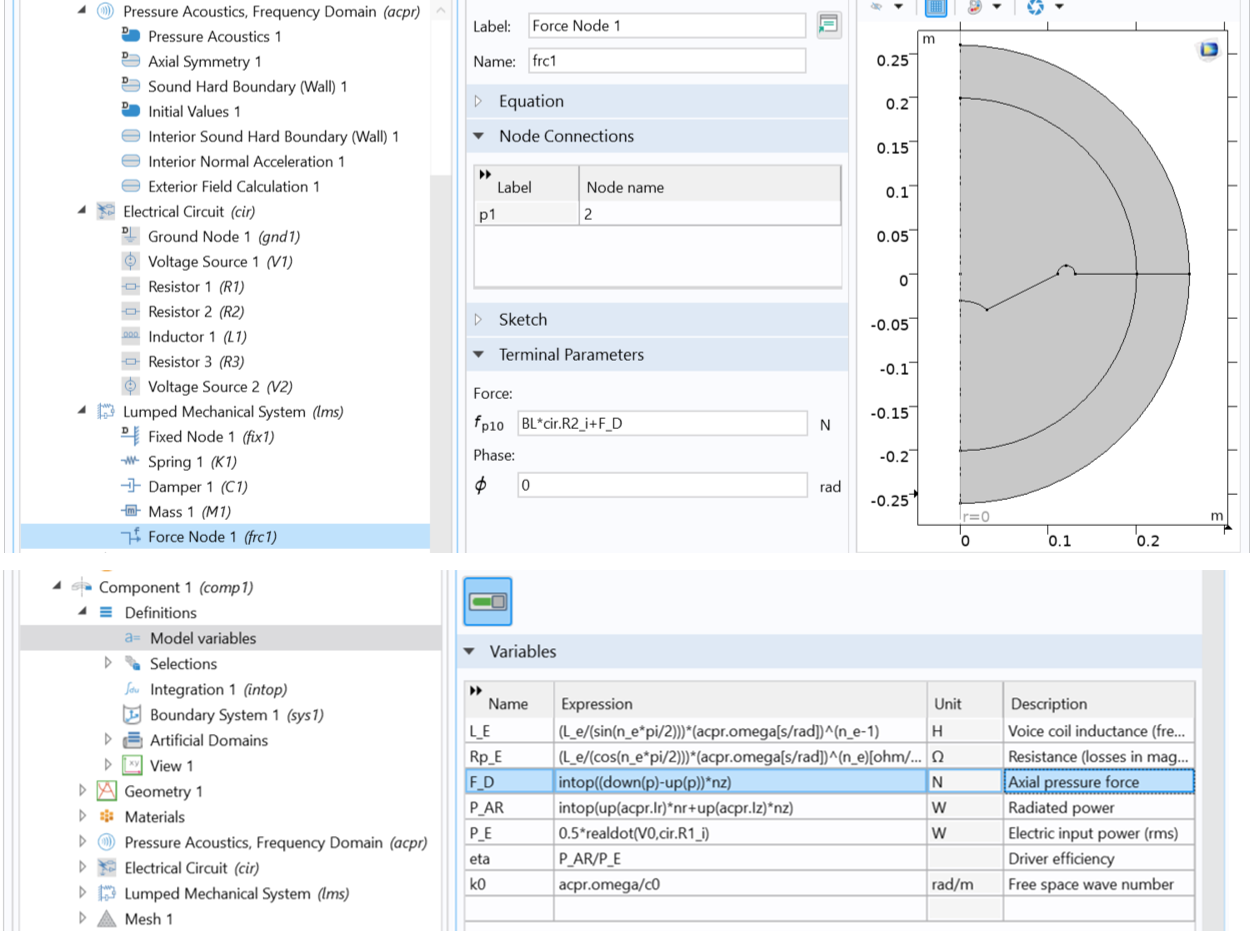A Force Node feature Settings window with the force defined by an equation and a table of variables with F_D highlighted.
The coil current from the electrical circuit model and the pressure drop across the diaphragm from the pressure acoustics model are passed to the lumped mechanical system for calculating the total force exerted on the mechanical system.

Further Learning

For exercises involving the lumped circuit and lumped mechanical model, download the following documentation and MPH-files from the Application Gallery: